Data structures with Go - Part II

Data Structures With Go - Part II

This page has been migrated to Medium

In the previous post we discussed how to implement linear data structures with Go.

Now we will explore two more complex data structures: tree and graph.

Those structures are not Linear and can represent unstructured information. Both graphs and trees are the foundation of the graph theory and both can be used, essentially, to describe a kind of relation.

In the domain of mathematics and computer science, graph theory is the study of graphs that concerns with the relationship among edges and vertices. It is a popular subject having its applications in computer science, information technology, biosciences and mathematics to name a few.

The structures we will develop are only for educational purpose, you should not use them in production, also because some of them are already implemented in the Go’s standard library.

None of those structures is thread-safe. We will make them thread-safe in future posts (I wish).

Let’s start by describing the most general one: the graph.

Graph

According to Wikipedia:

A graph data structure consists of a finite (and possibly mutable) set of vertices (also called nodes or points), together with a set of unordered pairs of these vertices for an undirected graph or a set of ordered pairs for a directed graph. These pairs are known as edges (also called links or lines), and for a directed graph are also known as arrows. The vertices may be part of the graph structure or may be external entities represented by integer indices or references.

So a graph is be a set $$G = (V,E)$$, where $$V$$ is a set of vertex (or nodes) and $$E$$ is a set of edges. We will focus on the undirected graph, but creating a directed graph from an undirected one is quite easy.

Graph

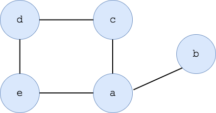
In the above graph, $$V = (a, b, c, d, e)$$ and $$E = ((a,b), (a,c), (c,d), (d,e), (e,a))$$.

For a more detailed (and theoretical) description of graphs and their application, you could read the book Algorithm Design.

Now it’s the coding time!

As usual, let’s start with defining our structures:

package graph

import (
	"fmt"
	"strings"
)

type Node struct {
	value interface{}
}

type Graph struct {
	nodes []*Node
	edges map[Node][]*Node
}

func NewGraph() *Graph {
	return &Graph{
		nodes: make([]*Node, 0),
		edges: make(map[Node][]*Node),
	}
}

As you can see from the code above, a Node is just a container for a value which is an interface{} so that we can use whatever type we want.

A Graph, instead, contains both an array of pointers to Nodes and a map which has Nodes as key and an array of pointers to Nodes as value.

This definition follows naturally the formal definition, so we defined a Graph as a pair of nodes and edges.

The NewGraph function only initializes nodes and edges.

Let’s see how to add nodes and edges:

func (g *Graph) AddNode(el interface{}) *Node {
	n := &Node{el}
	g.nodes = append(g.nodes, n)
	return n
}

func (g *Graph) AddEdge(n1, n2 *Node) {
	g.edges[*n1] = append(g.edges[*n1], n2)
	g.edges[*n2] = append(g.edges[*n2], n1)
}

Both the AddNode and AddEdge methods are easy to understand.

AddNode creates a Node which wraps the element, appends it to the node array and returns a pointer to that Node. This pointer can be useful next.

AddEdge takes two pointers to Nodes and appends them to the edge list in the map of each node.

func (n Node) String() string {
	return fmt.Sprintf("%v", n.value)
}

func (g Graph) String() string {
	sb := strings.Builder{}
	for _, v := range g.nodes {
		sb.WriteString(v.String())
		sb.WriteString(" -> [ ")
		neighbors := g.edges[*v]
		for _, u := range neighbors {
			sb.WriteString(u.String())
			sb.WriteString(" ")
		}
		sb.WriteString("]\n")
	}
	return sb.String()
}

The String method for the Node is trivial, while the String method for a Graph needs a explanation. We first create a strings.Builder which is the most efficient way to store a string incrementally. We then iterate over each Node and over each edge of that node. Let’s take the graph represented above: to create it in our code we could run the following snipped of code:

	g := NewGraph()
	nA := g.AddNode("a")
	nB := g.AddNode("b")
	nC := g.AddNode("c")
	nD := g.AddNode("d")
	nE := g.AddNode("e")

	g.AddEdge(nA, nB)
	g.AddEdge(nA, nC)
	g.AddEdge(nA, nE)
	g.AddEdge(nC, nD)
	g.AddEdge(nD, nE)

	fmt.Print(g.String())

Eventually, the Print statement will print the following:

a -> [ b c e ]
b -> [ a ]
c -> [ a d ]
d -> [ c e ]
e -> [ a d ]

Tree

According to Wikipedia:

In graph theory, a tree is an undirected graph in which any two vertices are connected by exactly one path, or equivalently a connected acyclic undirected graph. A forest is an undirected graph in which any two vertices are connected by at most one path, or equivalently an acyclic undirected graph, or equivalently a disjoint union of trees.

Generally speaking, a tree is a graph without cycles on which we could define a parent-children relationship.

The recursive definition of a tree is:

A tree is $$empty$$ or a vertex $$r$$ (the root of the tree) and a set of trees (the subtrees of $$T$$) whose roots are the children of $$r$$.

This definition helps us to understand the basic structure of a tree. So we could decompose a tree in many subtrees.

A tree is a collection of nodes connected by directed edges. It is a nonlinear data structure, compared to arrays, linked lists, stacks and queues which are linear data structures. A tree can be empty with no nodes or a tree is a structure consisting of one node called the root and zero or one or more subtrees. A tree has the following general properties:

one node is distinguished as a root;
every node but the root is connected by a directed edge from exactly one other node;
a direction is: $$parent \rightarrow children$$

Tree

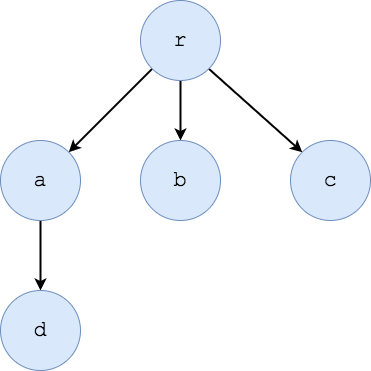
In the above tree we have a root $$r$$ having $$a$$, $$b$$ and $$c$$ as child. Subtrees of this tree are:

($$a$$, $$d$$), having $$a$$ as the root and $$d$$ as child of $$a$$;
$$b$$, having $$b$$ as the root and the empty tree as child of $$b$$;
$$c$$, having $$c$$ as the root and the empty tree as child of $$c$$;
$$d$$, having $$d$$ as the root and the empty tree as child of $$d$$.

For a more detailed (and theoretical) description of trees and their application, you could read the book Algorithm Design.

Now let’s translate this formal definition into code:

package tree

type Tree struct {
	el 		interface{}
	child 	[]*Tree
}

func (t *Tree) AddChild(el interface{}) *Tree {
	c := &Tree{el: el}
	t.child = append(t.child, c)
	return c
}

Code for Tree is quite easy, isn’t it?

Just think about the formal definition and see how we translate it in code:

A Tree struct contains an element el and a set (an array) of other Trees (child). When we add a child to a Tree using the AddChild method we create a new Tree with el as the element and no child, then we append this tree to the root.

To represent the above tree, we could run the following snippet:

	t := Tree{el: "r"}
	a := t.AddChild("a")
	a.AddChild("d")
	t.AddChild("b")
	t.AddChild("c")

Since this implementation is too easy, we’ll see how to implement the search using both BFS (breadth-first search) and DFS (depth-first search).

BFS

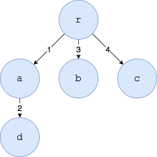
The BFS algorithm visits our tree level by level. A possible visit to our tree could be the following:

BFS

Labels on the edges represent the order of visit.

The code for a BFS visit is the following:

func (t *Tree) BFS(f func(*Tree)) {
	q := queue.Queue{}
	q.Enqueue(t)
	for !q.Empty() {
		next := q.Dequeue()
		nextNode := next.(*Tree)
		f(nextNode)
		if len(nextNode.child) > 0 {
			for _, child := range nextNode.child {
				q.Enqueue(child)
			}
		}
	}
}

We create a queue containing all the nodes to be visited. The first node added is obviously t (the root). A for iterates over the queue and applies the function f passing the dequeued element next. After visiting the element next, its child will be added to the queue.

To print our tree using BFS we can run:

	t.BFS(func(c *Tree) {
		fmt.Println(c.el)
	})

This will print:

r
a
b
c
d

DFS

The DFS algorithm visits each node of the tree trying to Go as deep as he can, then backtracking when encounters a node with no children (a leaf). A possible visit to our tree could be the following:

DFS

Code for DFS is far more elegant that the one for BFS since it uses recursion:

func (t *Tree) DFS(f func(*Tree)) {
	f(t)
	if len(t.child) > 0 {
		for _, c := range t.child {
			c.DFS(f)
		}
	}
}

It first calls f passing t, then visits each child of t and calls DFS on each one.

To print our tree using BFS we can run:

	t.DFS(func(c *Tree) {
		fmt.Println(c.el)
	})

This will print

r
a
d
b
c

Conclusion

Graphs and trees are powerful data structures since they allow you to store efficiently your data and their relationships. In literature, you can find so many different kinds of graphs and trees. A dept known of those structures makes you a better developer.

“The question of whether a computer can think is no more interesting than the question of whether a submarine can swim.”

Edsger W. Dijkstra